Common Geographical Database Operations

Feature Selection

It may be necessary to separate or to combine Attributes or Features before you can make the proper selection. Data can be selected as follows:

From the map view;
By overlaying data, then selecting particular Features from one theme based on how the Features relate to the Features of another theme;
By using a query to automatically select items from a table: this is accomplished by selecting the right Feature Type Code, Attribute Type Code and Attribute Value Code.

Example: To select all lakes for a dataset, you would select the records with Feature Code "4310" from the FEATTYP Attribute of the Water Area Geometry table (wa). From that subset select TYP Attribute Value Code ="2" for the Water Attribute Type, indicating a lake.

Table Joins

The following types of table joins are permissable:

Geometry tables can be joined with Attribute tables;
Attribute tables can be joined with other Attribute tables.

Two Geometry tables cannot be joined together.

Two or more tables can be linked based on a common reference feature. You can join two tables by an exact-match link of a unique record identifier in one table to one or more of the unique record identifiers in another table. A record identifier is a field such as a Feature ID. A record identifier can identify one or more records in a table.

Spatial Joins

A spatial join combines two or more Features, based on their geographical information. A spatial join is similar to an attribute join but is based on the spatial relationship between the Features (e.g., nearby, adjacent, inside or outside). As such, one Feature's records are joined into another Feature's basic Attribute table based on whether the Features' geometries correspond with a certain spatial relationship.

Example: When the roads in one Administrative Area are connected across the border with the roads in an adjacent Administrative Area, each road is connected spatially (the databases are "seamed"). The roads are physically connected, as they are in the real world. The Attributes of the road on one side of the border are available to the road on the other. This connection is necessary for routing.

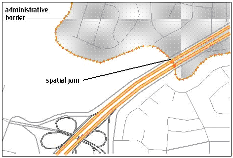
Figure: Spatial Joins

Joining Partitions: Features and Relationships that Cross Partitions

Features

All Features on partition borders are delivered in all adjacent partitions with their complete Attribute set.
A Feature that crosses a partition is split on the border. The Feature contains its complete Attribute set in all partitions.
When joining adjacent partitions, a geometrical join of the Features with the same Feature ID and Feature Type code results in the complete Feature containing all its Attributes.

Relationships

A Relationship that crosses a partition contains all Features, with their complete Attribute set, within the Relationship as if all Features that are referenced by the Relationship were present in that partition.
Example: A Parking Facility that belongs to a Shopping Center in another partition will result in a complete functional Relationship record in the Parking Facility's partition, even though the Shopping Center is not physically present in the Parking Facility's partition.
A Relationship that is built of multiple referencing records contains only the records that have at least one of the references present in the partition.
When joining neighboring partitions, the records of the Relationship have to be added in the same Feature Relationship. All double references have to be removed afterwards. There is no need to update fields in one of the Relationship records.

Summary and Dissolve

Summary and dissolve operations are manipulations that can affect your data more permanently than using the join operations.

A summary of data (also known as an "aggregation") can be both tabular and geographic.

A dissolve selects one or more areas, then dissolves the boundaries between them to make a larger area that includes the total information of all the areas. For non-adjacent areas like exclaves, just the Attribute information is appended.

The above definitions roughly depict the scope of the basic operations involved in any GIS project. However, the approach and algorithms behind these operations vary over the wide range of available GIS packages. For more information on the details of these basic operations, please see the manuals and user guides for your specific GIS package.